
Example 15.9. Volume Obtained by Rotating a Region about a Horizontal Axis.
In this example, we will determine the volume of the solid obtained by revolving the region bounded by \(y=x^2-4\) and \(y=-x^2+4\) about \(y=4\text{.}\)
It is a good idea to begin by plotting the two-dimensional region to help find the intersection points of the two curves.
> plot( [-x^2+4, x^2-4], x=-2..2, colour=[red, blue]);

As we can see from the graph, the intersection points occur at \((-2,0)\) and \((2,0)\text{.}\) This is easy to confirm by solving the system of two equations for \(x\) and \(y\text{.}\) This can be done with a single
solve() or fsolve() command, as explained in Example 10.2.
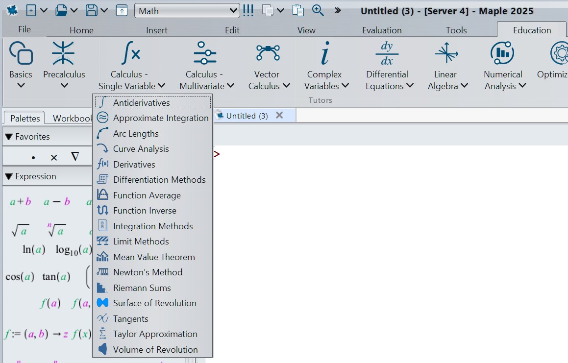
Now we can load up the Volume of Revolution tutor and enter the functions. When typing out the function in the tutor, you will not have access to the palettes toolbar in Maple, so you will need to type out commands such as
sqrt() for square roots and include the symbol * for multiplication. Be sure to set the correct variable and interval for the variable along with the information about the axis of revolution.
In this case, the Line of Revolution should be set to Horizontal, with a distance from the \(x\)-axis as \(4\text{.}\) Click Display when you have everything set up correctly.

It’s a good idea to copy the code in the Maple Command box at the bottom of the tutor so that it can be pasted into a new Maple input in your worksheet. This code uses the
VolumeOfRevolution() command, which has many options that may be changed to give various types of output. You can use this command to simply output the 3D graph of the solid:
> with(Student[Calculus1]):
> VolumeOfRevolution(-x^2+4, x^2-4, -2..2, 'axis'=horizontal,
    'distancefromaxis' = 4, 'showvolume'=true, 'showsum'=false,
    'showregion'=false, 'method'=midpoint, 'partition'= 6,
    'output'=plot);

Changing the
output option will can give you the exact value of the volume or the integral used to obtain the volume.
> VolumeOfRevolution(-x^2+4, x^2-4, -2..2, 'axis'=horizontal,
    'distancefromaxis' = 4, 'showvolume'=true, 'showsum'=false,
    'showregion'=false, 'method'=midpoint, 'partition'= 6,
    'output'=integral);
\begin{equation*}
\displaystyle \int_{-2}^{2}\! \,\pi\,\left((x^2-8)^{2}-x^4\right)\,{ d}x
\end{equation*}
> VolumeOfRevolution(-x^2+4, x^2-4, -2..2, 'axis'=horizontal,
    'distancefromaxis' = 4, 'showvolume'=true, 'showsum'=false,
    'showregion'=false, 'method'=midpoint, 'partition'= 6,
    'output'=value);
\begin{equation*}
\displaystyle {\frac {512\,\pi}{3}}
\end{equation*}
From this code, you can also easily change other options, such as the
axis (horizontal or vertical) and distancefromaxis.

